Key Takeaways
Performance Ratio links solar resource with delivered AC energy. A PR of 0.82 means the meter recorded 82% of the reference energy.
PVGIS’s 14% input covers one layer of the energy reduction. Temperature and incidence-angle effects are calculated separately.
Loss percentages compound through the energy path. Adding them directly overstates the combined reduction.
Loss patterns require different responses. Light-induced degradation occurs near the start of module operation, while soiling returns with site conditions and availability loss follows outages.
Project Builder combines cable, inverter and module losses. The resulting percentage replaces the PVGIS default and requires documented project assumptions.
What Performance Ratio Measures
Performance Ratio uses the two energy figures from the introduction. The 950 MWh is reference energy, calculated from plane-of-array irradiation and installed DC capacity at a reference irradiance of 1 kW/m². The AC meter supplies the delivered energy of 779 MWh.
Performance Ratio = Delivered AC energy ÷ Reference energy
Reference energy = Plane-of-array irradiation × Installed capacity ÷ 1 kW/m²
For the example:
779 MWh ÷ 950 MWh = 0.82
A PR of 0.82 means the array delivered 82% of its reference energy.
Module efficiency measures the share of incident sunlight converted to electricity under stated test conditions. Module area and efficiency determine rated power, expressed in Wp or kWp. Capacity factor compares annual production with continuous operation at rated capacity for 8,760 hours, so local irradiation influences the result. PR normalises production for available irradiation and focuses the assessment on system performance.
The PVGIS loss input covers selected system losses. PVGIS applies this percentage after modelling temperature and irradiance effects, placing the 14% default within the full PR reduction. IEC 61724-1 sets out the monitoring terminology and assessment methods.
The Loss Stack, Step by Step
Performance Ratio tells us how much reference energy reached the AC meter. The loss stack accounts for the remainder by following energy from the module surface through the DC and AC system. Availability then accounts for production missed during outages.
| Loss | Indicative planning range | Where it occurs | Pattern |
|---|---|---|---|
| Soiling | 1–5% | Dust or dirt blocks sunlight at the module surface | Seasonal and recurring |
| Temperature | 3–8% | Cell temperature rises above its reference condition | Weather-dependent |
| Light-induced degradation | 1–2% | Module output stabilises after initial light exposure | Initial |
| Long-term degradation | Around 0.5% per year | Module power declines with age | Progressive |
| Module mismatch | 1–2% | Modules or strings operate at different current-voltage points | Recurring |
| DC wiring | 1–2% | Resistance between the array and inverter | Recurring |
| Inverter conversion | 2–4% | Faults, maintenance or grid outages stop production | Recurring |
| AC wiring and connections | 0.5–1% | Resistance between the inverter and meter | Recurring |
| Availability loss | 0.5–3% | Faults, maintenance or grid outages stop production | Intermittent |
These ranges support project planning rather than direct addition. A combined loss budget applies them in sequence, as the next section explains.
Sunlight first reaches the module glass, where dust reduces the irradiation passing to the cells. Local dust conditions, rainfall, module tilt and cleaning frequency therefore set the soiling allowance. Once the cells receive this energy, their operating temperature affects DC output. Restricted airflow behind the array raises cell temperature and increases the reduction.
Light-induced degradation occurs near the start of module operation, following first exposure to sunlight. Long-term degradation develops over years. Separating these timescales prevents the initial reduction from reappearing as an annual rate.
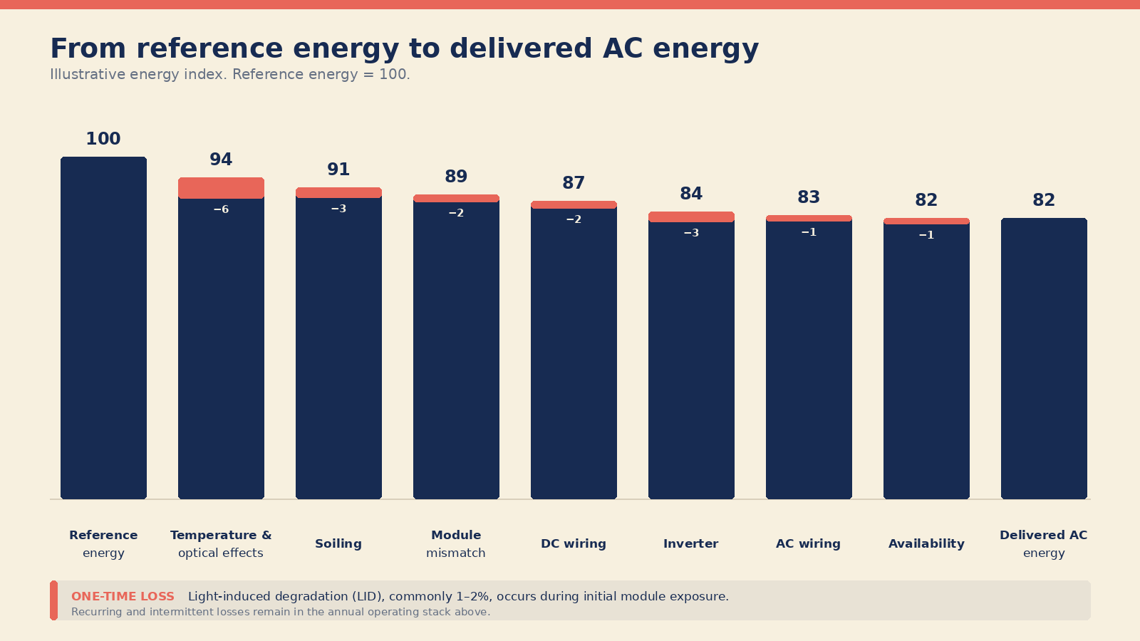
The remaining DC electricity passes through connected modules and cables. Differences in current and voltage create mismatch. Cable resistance dissipates part of the electrical energy as heat:
Cable power loss = Current² × Resistance
After the DC cables, the inverter converts the remaining energy to AC. Its efficiency varies with loading and input voltage, linking the conversion loss to equipment selection and operating conditions. Resistance in AC cables and connections dissipates another share on the way to the meter.
Availability loss falls outside this electrical path. A fault, maintenance period or grid outage removes production for part of the year. PVsyst separates optical, array and system losses in its energy balance, linking the final PR to individual causes.
A Realistic Loss Budget
The previous section identified the losses one by one. A project budget combines them in sequence. NREL’s PVWatts default values form the first column, while the second illustrates a project with reduced losses.
| Loss category | PVWatts reference | Optimised project example |
|---|---|---|
| Soiling | 2.0% | 1.0% |
| Shading | 3.0% | 0.5% |
| Mismatch | 2.0% | 1.0% |
| Wiring | 2.0% | 1.0% |
| Connections | 0.5% | 0.3% |
| Light-induced degradation | 1.5% | 1.0% |
| Nameplate tolerance | 1.0% | 0.5% |
| Availability | 3.0% | 1.0% |
Straight addition places the PVWatts entries at 15%. Their combined effect is lower because successive percentages apply to a shrinking energy balance:
Combined loss = 1 − [(1 − L₁) × (1 − L₂) × … × (1 − Lₙ)]
Applied to the PVWatts column:
1 − (0.98 × 0.97 × 0.98 × 0.98 × 0.995 × 0.985 × 0.99 × 0.97) = 14.08%
The optimised example produces a combined loss of 6.13%. Reduced shading, closer module matching and shorter downtime support this result. A project claiming this percentage requires evidence from its layout, equipment specifications and maintenance plan.
These totals cover only the categories listed in the table. PVWatts calculates module temperature and inverter conversion elsewhere in its model. PVGIS follows a related sequence: it calculates incidence-angle, temperature and irradiance effects, then applies the system-loss percentage. Its 14% input therefore covers one part of the energy reduction, while PR reflects the full result.
Which Losses Can Be Reduced?
The 6.13% budget depends on specific engineering and operating measures. A lower allowance requires project evidence.
| Loss | Main response |
|---|---|
| Soiling | Cleaning plan, module tilt and site maintenance |
| Mismatch | Module sorting and string design |
| DC/AC wiring | Cable sizing, shorter routes and sound terminations |
| Inverter | Equipment selection and suitable loading |
| Availability | Monitoring, spare parts and maintenance response |
| Temperature | Ventilated mounting and module temperature coefficient |
| Light-induced degradation | Module technology and procurement specification |
| Long-term degradation | Product qualification and supplier performance data |
Design choices influence wiring, mismatch and inverter losses. A larger conductor area cuts resistance, though extra copper raises capital cost. The investment becomes economical once recovered energy offsets the added expense.
Maintenance determines much of the soiling and availability allowance. Cleaning removes deposits but consumes labour and water. Monitoring shortens fault detection time, while spare parts reduce repair delays.
Site weather sets the operating conditions behind temperature loss. Ventilated mounting limits heat buildup, and a favourable temperature coefficient reduces the power penalty at high cell temperatures. Procurement choices also influence initial light-induced degradation and ageing over the project life.
Cable schedules and equipment datasheets support the design assumptions. Cleaning logs and outage records support the operating values. These records form the evidence behind the Project Builder inputs.
Setting Honest Loss Inputs in the Project Builder
The evidence gathered in the previous section informs three Project Builder entries: Cabling, Inverter and PV modules. Their current defaults are 1.0%, 2.0% and 0.5%, producing a combined input of 3.5%.

The Project Builder adds the three entries and sends the result to PVGIS through its loss parameter. This value replaces the PVGIS 14% default for the calculation. PVGIS therefore receives one system-loss percentage.
Temperature and irradiance response are modelled before PVGIS applies the submitted loss input. Adding temperature under PV modules counts the effect twice. Long-term degradation also belongs outside this field because the Project Builder applies a 0.5% annual degradation rate in its financial projection.
An example based on the available slider values is:
Cabling: 1.5%
Inverter: 2.5%
PV modules: 0.75%
Input sent to PVGIS: 4.75%
Run the calculation at the 3.5% starting value, then repeat it at 4.75% with the location and array settings unchanged. The resulting difference in annual yield reflects the additional 1.25 percentage points of system loss.
The current interface has no separate controls for soiling, mismatch, light-induced degradation or availability. A project estimate using the three-field input therefore requires a record of included and excluded losses. Enter this allocation in the project comment. Where project evidence remains limited, the PVGIS 14% reference supplies a broader allowance. A lower percentage requires support from cable calculations, inverter data and documented module assumptions.
Test Your Project Losses
Place your project point on the SolarBrief Project Builder map. Review the default loss percentages for cables, the inverter and PV modules, then replace them with documented project assumptions. Recalculate the PVGIS yield and compare annual production against the starting estimate. Record the selected percentages alongside the result for later project review.
FAQ
They cover different boundaries. Module efficiency measures the share of sunlight converted into DC electricity at the module. Performance Ratio compares delivered AC energy with reference energy based on irradiation and installed capacity, capturing losses across the operating system.
The 14% input represents one loss layer. PVGIS models incidence-angle, temperature and irradiance effects separately, then applies the system-loss percentage. The final PR reflects all these reductions.
PVGIS already models temperature using the module technology and mounting arrangement. Adding a temperature allowance to the loss fields counts that effect twice and understates the projected yield.
Glossary: Key Terms
| Term | Meaning |
|---|---|
| Reference energy | Theoretical energy from plane-of-array irradiation and installed DC capacity. Reference energy = Plane-of-array irradiation × Installed capacity ÷ 1 kW/m² |
| Performance Ratio (PR) | Share of reference energy recorded as delivered AC energy. PR = Delivered AC energy ÷ Reference energy |
| Plane-of-array irradiation | Solar energy reaching the tilted surface of the PV modules over a stated period. |
| Module efficiency | Share of incident solar energy converted to DC electricity by a module under stated conditions. |
| System loss | Energy reduction linked to equipment, wiring, soiling, outages or other operating conditions. |
| Derating factor | Percentage reduction applied to rated output to account for expected operating losses. |
| Temperature loss | Reduction in module power as cell temperature rises above its rated test condition. |
| Optical loss | Solar energy lost through reflection or an unfavourable angle between sunlight and the module surface. |
| Soiling loss | Irradiation blocked by dust, dirt or other deposits on the module glass. |
| Module mismatch | Output reduction caused by electrical differences between connected modules or strings. |
| DC wiring loss | Resistive loss between the modules and inverter. Cable power loss = Current² × Resistance |
| Inverter loss | Energy lost during conversion from direct current to alternating current. |
| AC wiring loss | Resistive loss between the inverter output and the delivery point. |
| Availability loss | Production missed during faults, maintenance or grid outages. |
| Light-induced degradation (LID) | Initial reduction in module output after first exposure to sunlight. |
| Long-term degradation | Gradual decline in module output over years of operation. |
| Combined loss | Total effect of several loss percentages applied in sequence. Combined loss = 1 − [(1 − L₁) × (1 − L₂) × … × (1 − Lₙ)] |
| PVGIS system-loss input | Percentage sent to PVGIS for user-assigned system losses. Project Builder combines its cable, inverter and module entries into this value. |
What it means
Performance Ratio compares delivered AC energy with the reference energy available to a PV array. SolarBrief’s Project Builder combines cable, inverter and module losses into one input for PVGIS. Documented project data supports a stronger estimate than a default percentage.
Sources: PVGIS 5 User Manual, PVGIS Data Sources and Calculation Methods, NREL PVWatts Version 5 Manual, IEC 61724-1:2021, PVsyst Performance Ratio, PVsyst Array and System Losses, PVsyst Ohmic Losses